Conclusions

Types of efficiency of investment projects

The following types of efficiency are distinguished:

– effectiveness of the project as a whole:

– effectiveness of participation in the project.

Overall project effectiveness is assessed to determine the potential attractiveness of the project for possible participants and to search for sources of financing. It includes:

– public (socio-economic) efficiency;

– commercial efficiency.

Efficiency of participation in the project is determined in order to verify its financial feasibility and the interest of all its participants in it and includes:

– efficiency for participating enterprises ;

– efficiency for shareholders ;

– efficiency for higher-level structures (national economic and regional, sectoral, budgetary).

Basic principles for assessing the effectiveness of investment projects:

– consideration of the project throughout its entire life cycle (calculation period);

– cash flow modeling;

– comparability of conditions for comparing different projects (project options);

– the principle of positivity and maximum effect;

– taking into account the time factor;

– accounting only for upcoming costs and revenues;

– taking into account the most significant consequences of the project;

– taking into account the interests of different project participants;

– multi-stage assessment;

– taking into account the impact of uncertainty and risks.

Evaluating the effectiveness of investment projects is usually carried out in two stages:

At the first stage efficiency indicators of the project as a whole are calculated. For local projects, only their commercial effectiveness is assessed and, if it turns out to be acceptable, they move on to the second stage of assessment.

Second stage carried out after determining the financing scheme. At this stage, the composition of participants is clarified and the financial feasibility and effectiveness of participation in the project of each of them is determined.

Features of efficiency assessment at different stages of project development are that:

– at the stages of searching for investment opportunities and preliminary preparation of the project, as a rule, they are limited to assessing the effectiveness of the project as a whole, while cash flow calculations are made in current prices. Initial data are determined on the basis of analogy, expert assessments, and average statistical data. The calculation step is usually taken to last one year;

– at the stage of final preparation of the project, all of the above types of efficiency are assessed. In this case, real initial data should be used, including the financing scheme, and calculations should be made in current, forecast and deflated prices.

Purpose of definition financing schemes – provision financial feasibility investment project. Ignoring uncertainty and risk, then a sufficient condition for the financial feasibility of an investment project is the non-negativity at each step of the value of the accumulated balance of the flow.

Economic assessment of investment projects occupies a central place in the process of justification and selection of possible options for investing in real assets. Despite all the other favorable characteristics of the project, it will be rejected if it does not provide:

– reimbursement of invested funds from income from the sale of goods or services;

– obtaining a profit that ensures a return on investment not lower than the level desired for the enterprise;

– return on investment within a period acceptable for the enterprise.

Time value of money

In its most general form, the meaning of the concept “time value of money” can be expressed by the phrase - a ruble today is worth more than the ruble that we will receive in the future. A ruble received today can be immediately invested in business, and it will generate profit. Or you can put it in a bank account and earn interest.

Compound interest formula: ,

where FV is the future value of the amount that we invest in any form today and which we will have over the period of time we are interested in;

PV is the current (modern) value that we invest;

E – the amount of return on investment;

k – the number of time periods during which the investment will participate in commercial circulation.

From the above formula it is clear that to calculate the future value ( F.V. ) compound interest is applied. This means that the interest accrued on the original amount is added to that original amount and interest is also charged on it.

Discounting

To determine the current (modern) value (PV) of future income and expenses, we use the compound interest formula:

.

Therefore, the current (modern) value is equal to the future value multiplied by the coefficient
, called the discount factor.

Discounting is the process of bringing (adjusting) the future value of money to its current (modern) value.

Future value of the annuity

Annuity – this is a special case of cash flow, i.e. This is a flow in which cash receipts (or payments) in each period are the same in size.

,

where FVA k is the future value of the annuity;

PMT t – payment made at the end of the period;

E – income level;

k is the number of periods during which income is generated.

The current value of the annuity is determined by the formula :

,

where PMT t is future cash receipts at the end of the period;

E – rate of return on investments;

k is the number of periods during which future income from modern investments will be received.

Discount factor. Discount rate

Discounting cash flows is the reduction of their values ​​at different times to their value at a certain point in time, which is called moment of bringing and is denoted by .

The moment of reduction may not coincide with the beginning of the time count, t 0 . The discounting procedure is understood in an expanded sense, i.e. as a reduction not only to an earlier point in time, but also to a later one (if
).

The main economic standard used in discounting is the discount rate (E).

Discounting of cash flow at the m-th step is carried out by multiplying its NPV value m (CF m) by the discount factor (), calculated by the formula

,

where t m is the moment of the end of the mth calculation step.

Discount rate from an economic point of view –It is the rate of return that an investor would typically receive from an investment of similar content and degree of risk. So this is the expected rate of return.

The following discount rates are distinguished:

– commercial;

– project participant;

– social;

- budget.

Commercial discount rate determined taking into account alternative efficiency of capital use.

Project participant discount rate chosen by the participants themselves.

To assess the commercial effectiveness of the project as a whole, foreign financial management experts recommend using a commercial discount rate set at cost of capital. The total amount of funds that must be paid for the use of financial resources to their owners (dividends, interest) as a percentage of their volume is called cost of capital .

If the investment project is carried out at the expense of the enterprise’s own capital, then the commercial discount rate (for the effectiveness of the project as a whole) can be established in accordance with the requirements for the minimum acceptable future profitability, determined depending on the deposit rates of banks of the first reliability category.

In the economic assessment of investment projects carried out at the expense of borrowed funds, the discount rate is assumed to be equal to the interest rate on the loan.

In the case of mixed capital (equity and debt capital), the discount rate is determined as the weighted average cost of capital:

,

where n is the number of types of capital;

E i – discount rate of i-th capital;

d i is the share of the i-th capital in the total capital.

Risk-adjusted discount rate

Depending on the method of taking into account the uncertainty of the conditions for the implementation of an investment project when determining the net present value, the discount rate in efficiency calculations may or may not include a risk adjustment. Risk adjustment is usually made when a project is being evaluated or under a single scenario for its implementation.

The risk adjustment value generally takes into account three types of risks associated with the implementation of an investment project:

country risk;

the risk of unreliability of project participants;

the risk of not receiving the income provided for by the project.

Accounting for changes in the discount rate over time

First of all, this is due to the improvement of the financial markets of Russia, as a result of which the refinancing rate of the Central Bank of Russia is reduced.

The need to take into account changes in the discount rate by steps of the calculation period may also be determined by the method of establishing this rate. Thus, when using a commercial discount rate set at the weighted average cost of capital (WACC), as the capital structure and dividend policy change, the WACC will change.

Discounting cash flows with a discount rate changing over time differs, first of all, in the calculation formula for determining the discount rate:

,

where E 0 , ..., E m are the discount rates at the 0th, ..., mth steps, respectively,

 0 ,…, m – the duration of these steps in years or fractions.

"

Highly specialized material for professional investors
and students of the Fin-plan course "".

Financial and economic calculations most often involve the assessment of cash flows distributed over time. Actually, for these purposes a discount rate is needed. From the point of view of financial mathematics and investment theory, this indicator is one of the key ones. It is used to build methods of investment valuation of a business based on the concept of cash flows, and with its help, a dynamic assessment of the effectiveness of investments, both real and stock, is carried out. Today, there are already more than a dozen ways to select or calculate this value. Mastering these methods allows a professional investor to make more informed and timely decisions.

But, before moving on to methods for justifying this rate, let’s understand its economic and mathematical essence. Actually, two approaches are used to define the term “discount rate”: conventionally mathematical (or process), and economic.

The classic definition of the discount rate comes from the well-known monetary axiom: “money today is worth more than money tomorrow.” Hence, the discount rate is a certain percentage that allows you to reduce the value of future cash flows to their current cost equivalent. The fact is that many factors influence the depreciation of future income: inflation; risks of non-receipt or shortfall of income; lost profits that arise when a more profitable alternative opportunity to invest funds appears in the process of implementing a decision already made by the investor; systemic factors and others.

By applying the discount rate in his calculations, the investor brings or discounts expected future cash income to the current point in time, thereby taking into account the above factors. Discounting also allows the investor to analyze cash flows distributed over time.

However, one should not confuse the discount rate and the discount factor. The discount factor is usually operated in the calculation process as a certain intermediate value, calculated on the basis of the discount rate using the formula:

where t is the number of the forecast period in which cash flows are expected.

The product of the future cash flow and the discount factor shows the current equivalent of the expected income. However, the mathematical approach does not explain how the discount rate itself is calculated.

For these purposes, the economic principle is applied, according to which the discount rate is some alternative return on comparable investments with the same level of risk. A rational investor, making a decision to invest money, will agree to implement his “project” only if its profitability turns out to be higher than the alternative one available on the market. This is not an easy task, since it is very difficult to compare investment options by risk level, especially in conditions of lack of information. In the theory of investment decision making, this problem is solved by decomposing the discount rate into two components - the risk-free rate and risks:

The risk-free rate of return is the same for all investors and is subject only to the risks of the economic system itself. The investor assesses the remaining risks independently, usually based on expert assessment.

There are many models for justifying the discount rate, but they all correspond in one way or another to this basic fundamental principle.

Thus, the discount rate always consists of the risk-free rate and the total investment risk of a particular investment asset. The starting point in this calculation is the risk-free rate.

Risk-free rate

The risk-free rate (or risk-free rate of return) is the expected rate of return on assets for which their own financial risk is zero. In other words, this is the yield on absolutely reliable investment options, for example, on financial instruments whose profitability is guaranteed by the state. We emphasize that even for absolutely reliable financial investments, absolute risk cannot be absent (in this case, the rate of return would tend to zero). The risk-free rate precisely includes risk factors of the economic system itself, risks that no investor can influence: macroeconomic factors, political events, changes in legislation, emergency man-made and natural events, etc.

Therefore, the risk-free rate reflects the minimum possible return acceptable to the investor. The investor must choose the risk-free rate for himself. You can calculate the average bet from several potentially risk-free investment options.

When choosing a risk-free rate, an investor must take into account the comparability of his investments with the risk-free option according to such criteria as:

The scale or total cost of the investment.

Investment period or investment horizon.

The physical possibility of investing in a risk-free asset.

Equivalence of denominated rates in foreign currency, and others.

Return rates on time ruble deposits in banks of the highest reliability category. In Russia, such banks include Sberbank, VTB, Gazprombank, Alfa-Bank, Rosselkhozbank and a number of others, a list of which can be viewed on the website of the Central Bank of the Russian Federation. When choosing a risk-free rate using this method, it is necessary to take into account the comparability of the investment period and the period for fixing the deposit rate.

Let's give an example. Let's use the data from the website of the Central Bank of the Russian Federation. As of August 2017, the weighted average interest rates on deposits in rubles for up to 1 year were 6.77%. This rate is risk-free for most investors investing for up to 1 year;

Yield level on Russian government debt financial instruments. In this case, the risk-free rate is fixed in the form of the yield on (OFZ). These debt securities are issued and guaranteed by the Ministry of Finance of the Russian Federation, and therefore are considered the most reliable financial asset in the Russian Federation. With a maturity of 1 year, OFZ rates currently range from 7.5% to 8.5%.

Yield level on foreign government securities. In this case, the risk-free rate is equal to the yield on US government bonds with maturities from 1 year to 30 years. Traditionally, the US economy is assessed by international rating agencies at the highest level of reliability, and, consequently, the yield of their government bonds is considered risk-free. However, it should be taken into account that the risk-free rate in this case is denominated in dollar rather than ruble equivalent. Therefore, to analyze investments in rubles, an additional adjustment is necessary for the so-called country risk;

Yield level on Russian government Eurobonds. This risk-free rate is also denominated in US dollars.

Key rate of the Central Bank of the Russian Federation. At the time of writing this article, the key rate is 9.0%. This rate is considered to reflect the price of money in the economy. An increase in this rate entails an increase in the cost of the loan and is a consequence of an increase in risks. This tool should be used with great caution, since it is still a guideline and not a market indicator.

Interbank lending market rates. These rates are indicative and more acceptable compared to the key rate. Monitoring and a list of these rates are again presented on the website of the Central Bank of the Russian Federation. For example, as of August 2017: MIACR 8.34%; RUONIA 8.22%, MosPrime Rate 8.99% (1 day); ROISfix 8.98% (1 week). All these rates are short-term in nature and represent the profitability of lending operations of the most reliable banks.

Discount rate calculation

To calculate the discount rate, the risk-free rate should be increased by the risk premium that the investor assumes when making certain investments. It is impossible to assess all risks, so the investor must independently decide which risks should be taken into account and how.

The following parameters have the greatest influence on the risk premium and, ultimately, the discount rate:

The size of the issuing company and the stage of its life cycle.

The nature of the liquidity of the company's shares on the market and their volatility. The most liquid stocks generate the least risk;

Financial condition of the issuer of shares. A stable financial position increases the adequacy and accuracy of forecasting the company's cash flow;

Business reputation and market perception of the company, investor expectations regarding the company;

Industry affiliation and risks inherent in this industry;

The degree of exposure of the issuing company’s activities to macroeconomic conditions: inflation, fluctuations in interest rates and exchange rates, etc.

A separate group of risks includes the so-called country risks, that is, the risks of investing in the economy of a particular state, for example Russia. Country risks are usually already included in the risk-free rate if the rate itself and the risk-free yield are denominated in the same currencies. If the risk-free return is in dollar terms, and the discount rate is needed in rubles, then it will be necessary to add country risk.

This is just a short list of risk factors that can be taken into account in the discount rate. Actually, depending on the method of assessing investment risks, the methods for calculating the discount rate differ.

Let's briefly look at the main methods for justifying the discount rate. To date, more than a dozen methods for determining this indicator have been classified, but they are all grouped as follows (from simple to complex):

Conventionally “intuitive” - based rather on the psychological motives of the investor, his personal beliefs and expectations.

Expert, or qualitative - based on the opinion of one or a group of specialists.

Analytical – based on statistics and market data.

Mathematical, or quantitative, require mathematical modeling and the possession of relevant knowledge.

An “intuitive” way to determine the discount rate

Compared to other methods, this method is the simplest. The choice of discount rate in this case is not mathematically justified in any way and represents only the investor’s desire, or his preference about the level of return on his investments. An investor can rely on his previous experience, or on the profitability of similar investments (not necessarily his own) if information about the profitability of alternative investments is known to him.

Most often, the discount rate is “intuitively” calculated approximately by multiplying the risk-free rate (as a rule, this is simply the rate on deposits or OFZ) by some adjustment factor of 1.5, or 2, etc. Thus, the investor, as it were, “estimates” the level of risks for himself.

For example, when calculating discounted cash flows and fair values ​​of companies in which we plan to invest, we typically use the following rate: the average deposit rate multiplied by 2 if we are talking about blue chips and use higher coefficients if we are talking about companies 2nd and 3rd echelons.

This method is the easiest for a private investor to practice and is used even in large investment funds by experienced analysts, but it is not held in high esteem among academic economists because it allows for “subjectivity.” In this regard, in this article we will give an overview of other methods for determining the discount rate.

Calculation of discount rate based on expert assessment

The expert method is used when investments involve investing in shares of companies in new industries or activities, startups or venture funds, and also when there is no adequate market statistics or financial information about the issuing company.

The expert method for determining the discount rate consists of surveying and averaging the subjective opinions of various specialists about the level, for example, of the expected return on a specific investment. The disadvantage of this approach is the relatively high degree of subjectivity.

You can increase the accuracy of calculations and somewhat level out subjective assessments by decomposing the bet into a risk-free level and risks. The investor chooses the risk-free rate independently, and the assessment of the level of investment risks, the approximate content of which we described earlier, is carried out by experts.

The method is well applicable for investment teams that employ investment experts of various profiles (currency, industry, raw materials, etc.).

Calculation of the discount rate using analytical methods

There are quite a lot of analytical ways to justify the discount rate. All of them are based on theories of firm economics and financial analysis, financial mathematics and business valuation principles. Let's give a few examples.

Calculation of the discount rate based on profitability indicators

In this case, the justification for the discount rate is carried out on the basis of various profitability indicators, which in turn are calculated based on data and. The basic indicator is return on equity (ROE, Return On Equity), but there may be others, for example, return on assets (ROA, Return On Assets).

Most often it is used to evaluate new investment projects within an existing business, where the nearest alternative rate of return is precisely the profitability of the current business.

Calculation of the discount rate based on the Gordon model (constant dividend growth model)

This method of calculating the discount rate is acceptable for companies paying dividends on their shares. This method presupposes the fulfillment of several conditions: payment and positive dynamics of dividends, no restrictions on the life of the business, stable growth of the company’s income.

The discount rate in this case is equal to the expected return on the company's equity capital and is calculated using the formula:

This method is applicable to evaluate investments in new projects of a company by shareholders of this business, who do not control profits, but only receive dividends.

Calculation of the discount rate using quantitative analysis methods

From the perspective of investment theory, these methods and their variations are the main and most accurate. Despite the many varieties, all these methods can be reduced to three groups:

Cumulative construction models.

Capital asset pricing models CAPM (Capital Asset Pricing Model).

WACC (Weighted Average Cost of Capital) models.

Most of these models are quite complex and require certain mathematical or economic skills. We will look at general principles and basic calculation models.

Cumulative construction model

Within this method, the discount rate is the sum of the risk-free rate of expected return and the total investment risk for all types of risk. The method of justifying the discount rate based on risk premiums to the risk-free level of return is used when it is difficult or impossible to assess the relationship between risk and return on investment in the business being analyzed using mathematical statistics. In general, the calculation formula looks like this:

CAPM Capital Asset Pricing Model

The author of this model is Nobel laureate in economics W. Sharp. The logic of this model is no different from the previous one (the rate of return is the sum of the risk-free rate and risks), but the method for assessing investment risk is different.

This model is considered fundamental because it establishes the dependence of profitability on the degree of its exposure to external market risk factors. This relationship is assessed through the so-called “beta” coefficient, which is essentially a measure of the elasticity of an asset’s return to changes in the average market return of similar assets on the market. In general, the CAPM model is described by the formula:

Where β is the “beta” coefficient, a measure of systematic risk, the degree of dependence of the assessed asset on the risks of the economic system itself, and the average market return is the average return on the market of similar investment assets.

If the “beta” coefficient is above 1, then the asset is “aggressive” (more profitable, changes faster than the market, but also more risky in relation to its analogues on the market). If the beta coefficient is below 1, then the asset is “passive” or “defensive” (less profitable, but also less risky). If the “beta” coefficient is equal to 1, then the asset is “indifferent” (its profitability changes in parallel with the market).

Calculation of discount rate based on WACC model

Estimating the discount rate based on the company's weighted average cost of capital allows us to estimate the cost of all sources of financing its activities. This indicator reflects the company's actual costs for paying for borrowed capital, equity capital, and other sources, weighted by their share in the overall liability structure. If a company's actual profitability is higher than the WACC, then it generates some added value for its shareholders, and vice versa. That is why the WACC indicator is also considered as a barrier value of the required return for the company’s investors, that is, the discount rate.

The WACC indicator is calculated using the formula:

Of course, the range of methods for justifying the discount rate is quite wide. We have described only the main methods most often used by investors in a given situation. As we said earlier in our practice, we use the simplest, but quite effective “intuitive” method of determining the rate. The choice of a specific method always remains with the investor. You can learn the entire process of making investment decisions in practice in our courses at. We teach in-depth analytical techniques already at the second level of training, in advanced training courses for practicing investors. You can evaluate the quality of our training and take your first steps in investing by signing up for our courses.

If the article was useful to you, like it and share it with your friends!

Profitable investments for you!

Let's touch on such a complex economic term as the discount rate, consider existing modern methods for calculating it and areas of use.

Discount rate and its economic meaning

Discount rate (analog: comparison rate, rate of return)- This is the interest rate that is used to reestimate the value of future capital at the current moment. This is done due to the fact that one of the fundamental laws of economics is the constant depreciation of the value (purchasing power, cost) of money. The discount rate is used in investment analysis when an investor decides about the prospect of investing in a particular object. To do this, he reduces the future value of the investment object to the present (current). By conducting a comparative analysis, he can decide on the attractiveness of the object. Any value of an object is always relative, so the discount rate acts as the basic criterion with which the effectiveness of an investment is compared. Depending on different economic objectives, the discount rate is calculated differently. Let's consider existing methods for estimating the discount rate.

Methods for estimating discount rates

Let's consider 10 methods for estimating the discount rate for evaluating investments and investment projects of an enterprise/company.

• Capital Asset Valuation Models CAPM;
• Modified capital asset valuation model CAPM;
• Model by E. Fama and K. French;
• Model M. Carhart;
• Constant Growth Dividend Model (Gordon);
• Calculation of discount rate based on weighted average cost of capital (WACC);
• Calculation of discount rate based on return on equity;
• Market multiplier method
• Calculation of discount rate based on risk premiums;
• Calculation of the discount rate based on expert assessment;

Calculation of discount rate based on the CAPM model

Capital Asset Pricing Model – CAPM ( CapitalAssetPricingModel) was proposed in the 70s by W. Sharp (1964) to estimate the future return on shares/capital of companies. The CAPM model reflects future returns as the return on a risk-free asset and a risk premium. As a result, if the expected return on a stock is lower than the required return, investors will refuse to invest in this asset. Market risk was taken as a factor determining the future rate in the model. The formula for calculating the discount rate using the CAPM model is as follows:

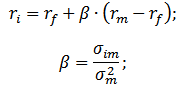where: r i – expected return on the stock (discount rate);

r f – return on a risk-free asset (for example: government bonds);

r m – market return, which can be taken as the average return on the index (MICEX, RTS - for Russia, S&P500 - for the USA);

β – beta coefficient. Reflects the riskiness of the investment in relation to the market, and shows the sensitivity of changes in stock returns to changes in market returns;

σ im – standard deviation of changes in stock returns depending on changes in market returns;

σ 2 m – dispersion of market returns.

Advantages and disadvantages of the CAPM capital asset pricing model

• The model is based on the fundamental principle of the relationship between stock returns and market risk, which is its advantage;
• The model includes only one factor (market risk) to estimate the future return of a stock. Researchers such as Y. Fama, K. French, and others have introduced additional parameters into the CAPM model to increase its forecasting accuracy.
• The model does not take into account taxes, transaction costs, opacity of the stock market, etc.

Calculation of the discount rate using the modified CAPM model

The main disadvantage of the CAPM model is its one-factor nature. Therefore, the modified capital asset pricing model also includes adjustments for unsystematic risk. Unsystematic risk is also called specific risk, which appears only under certain conditions. Calculation formula for modified CAPM model (ModifiedCapitalAssetPricingModel,MCAPM) is as follows:

where: r i – expected return on the stock (discount rate); r f – return on a risk-free asset (for example, government bonds); r m – market return; β – beta coefficient; σ im is the standard deviation of the change in stock returns from the change in market returns; σ 2 m – dispersion of market returns;

r u – risk premium, including the company’s unsystematic risk.

As a rule, experts are used to assess specific risks because they are difficult to formalize using statistics. The table below shows various risk adjustments ⇓.

Specific risks	Risk adjustment, %
Government influence on tariffs	0,4%
Changes in prices for raw materials, materials, energy, components, rent	0,2%
Management risk of the owner/shareholders	0,2%
Influence of Key Suppliers	0,3%
The influence of seasonality in demand for products	0,4%
Conditions for raising capital	0,3%
Total adjustment for specific risk:	1,8%

For example, let’s calculate the discount rate taking into account adjustments, so if according to the CAPM model the yield is 10%, then taking into account risk adjustments the discount rate will be 11.8%. Using a modified model allows you to more accurately determine the future rate of return.

Calculation of the discount rate using the model of E. Fama and K. French

One of the modifications of the CAPM model was the three-factor model of E. Fama and K. French (1992), which began to take into account two more parameters that influence the future rate of profit: company size and industry specifics. Below is the formula of the three-factor model of E. Fama and K. French:

where: r – discount rate; r f – risk-free rate; r m – profitability of the market portfolio;

SMB t is the difference between the returns of weighted average portfolios of small and large capitalization stocks;

HML t is the difference between the returns of weighted average portfolios of shares with large and small ratios of book value to market value;

β, si, h i – coefficients that indicate the influence of parameters r i, r m, r f on the profitability of the i-th asset;

γ is the expected return of an asset in the absence of the influence of 3 risk factors on it.

Calculation of the discount rate based on the M. Karhat model

The three-factor model of E. Fama and K. French was modified by M. Carhart (1997) by introducing a fourth parameter to assess the possible future return of a stock - moment. The moment reflects the rate of price change over a certain historical period of time; when the fourth parameter is used in the model for estimating the profitability of a stock in the future, it is taken into account that the future rate of return is also affected by the rate of price change. Below is the formula for calculating the discount rate using the M. Carhart model:

where: r – discount rate; WMLt – moment, rate of change in the value of a stock over the previous period.

Calculation of the discount rate based on the Gordon model

Another method for calculating the discount rate is to use the Gordon model (Constant Growth Dividend Model). This method has some limitations on its use, because in order to estimate the discount rate, it is necessary that the company issues ordinary shares with dividend payments. Below is the formula for calculating the cost of equity capital of an enterprise (discount rate):

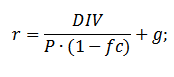Where:

DIV – the amount of expected dividend payments per share for the year;

P – share placement price;

fc – costs of issuing shares;

g – dividend growth rate.

Calculation of discount rate based on weighted average cost of capital WACC

Method for estimating the discount rate based on the weighted average cost of capital (eng. WACC, Weighted Average Cost of Capital) one of the most popular and shows the rate of return that should be paid for the use of investment capital. Investment capital can consist of two sources of financing: equity and debt. Often, WACC is used both in financial and investment analysis to estimate the future return on investment, taking into account the initial conditions for the return (profitability) of investment capital. The economic meaning of calculating the weighted average cost of capital is to calculate the minimum acceptable level of profitability (profitability, profitability) of the project. This indicator is used to evaluate investments in an existing project. The formula for calculating the weighted average cost of capital is as follows:

where: r e ,r d – expected (required) return on equity and debt capital, respectively;

E/V, D/V – share of equity and debt capital. The sum of equity and borrowed capital forms the company’s capital (V=E+D);

t – profit tax rate.

Calculation of discount rate based on return on equity

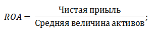
The advantages of this method include the ability to calculate the discount rate for enterprises that are not listed on the stock market. Therefore, to evaluate the discount, return on equity and debt capital indicators are used. These indicators are easily calculated from balance sheet items. If an enterprise has both equity and borrowed capital, then the indicator used is return on assets. (Return On Assets, ROA). The formula for calculating the return on assets ratio is presented below:

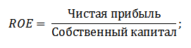
The next method for estimating the discount rate through return on equity is (Return On Equity, ROE), which shows the efficiency/profitability of capital management of an enterprise (company). The profitability ratio shows what rate of profit the company creates using its capital. The formula for calculating the coefficient is as follows:

Developing this approach in assessing the discount rate through assessing the return on capital of the enterprise, a more accurate indicator can be used as a criterion for assessing the rate - return on capital employed (ROCEReturnOnCapitalEmployed). This indicator, unlike ROE, uses long-term liabilities (through shares). This indicator can be used for companies that have preferred shares on the stock market. If the company does not have them, then the ROE ratio is equal to ROCE. The indicator is calculated using the formula:

Another type of return on equity ratio is return on average capital employed ROACE. (Return on Average Capital Employed).

In fact, this indicator corresponds to ROCE, its main difference is the averaging of the cost of capital employed (Equity + long-term liabilities) at the beginning and end of the period being assessed. The formula for calculating this indicator:

The ROACE indicator can often replace ROCE, for example, in the EVA economic value added formula. Let us present an analysis of the feasibility of using profitability ratios to estimate the discount rate ⇓.

Calculation of discount rate based on expert assessment

If you need to estimate the discount rate for a venture project, then using the CAPM, Gordon model and WACC methods is impossible, so experts are used to calculate the rate. The essence of expert analysis is the subjective assessment of various macro, meso and micro factors affecting the future rate of profit. Factors that have a strong influence on the discount rate: country risk, industry risk, production risk, seasonal risk, management risk, etc. For each individual project, experts identify their most significant risks and evaluate them using scoring. The advantage of this method is the ability to take into account all possible investor requirements.

Calculation of discount rate based on market multipliers

This method is widely used to calculate the discount rate for enterprises that issue ordinary shares on the stock market. As a result, the market E/P multiplier is calculated, which is translated as EBIDA/Price. The advantages of this approach are that the formula reflects industry risks when valuing a company.

Calculation of discount rate based on risk premiums

The discount rate is calculated as the sum of the risk-free interest rate, inflation and risk premium. As a rule, this method of estimating the discount rate is carried out for various investment projects where it is difficult to statistically estimate the amount of possible risk/return. Formula for calculating the discount rate taking into account the risk premium:

Where:

r – discount rate;

r f – risk-free interest rate;

r p – risk premium;

I – inflation percentage.

The discount rate formula consists of the sum of the risk-free interest rate, inflation and the risk premium. Inflation was singled out as a separate parameter because money depreciates constantly; this is one of the most important laws of economic functioning. Let us consider separately how each of these components can be assessed.

Methods for estimating the risk-free interest rate

To assess the risk-free value, financial instruments are used that provide profitability with zero risk, that is, absolutely reliable. In reality, no instrument can be considered absolutely reliable; it’s just that the probability of losing money when investing in it is extremely small. Let's consider two methods for estimating the risk-free rate:

1. Yield on risk-free government bonds (GKOs - government short-term zero-coupon bonds, OFZs - federal loan bonds) issued by the Ministry of Finance of the Russian Federation. Government bonds have the highest safety rating, so they can be used to calculate the risk-free interest rate. The yield on these types of bonds can be viewed on the website of the Central Bank of the Russian Federation (cbr.ru) and on average it can be taken as 6% per annum.
2. US 30-year bond yield. The average yield on these financial instruments is 5%.

Methods for estimating risk premium

The next component of the formula is the risk premium. Since risks always exist, their impact on the discount rate should be assessed. There are many methods for assessing additional investment risks; let’s look at some of them.

Methodology for assessing risk adjustments from the Alt-Invest company

The Alt-Invest methodology includes the following types of risks in the risk adjustment, presented in table ⇓.

Methodology of the Government of the Russian Federation No. 1470 (dated November 22, 1997) for assessing the discount rate for investment projects

The purpose of this methodology is to evaluate investment projects for public investment. Specific risks and adjustments for them will be calculated through expert assessment. To calculate the base (risk-free) discount rate, the refinancing rate of the Central Bank of the Russian Federation was used; this rate can be viewed on the official website of the Central Bank of the Russian Federation (cbr.ru). Specific project risks are assessed by experts in the presented ranges. The maximum discount rate using this method will be 61%.

Risk-free interest rate
WITH refinancing rate of the Central Bank of the Russian Federation	11%
Risk premium
Specific risks	Risk adjustment, %
Investments to intensify production	3-5%
Increasing product sales volume	8-10%
The risk of introducing a new type of product to the market	13-15%
Research costs	18-20%

Methodology for calculating the discount rate Vilensky P.L., Livshits V.N., Smolyak S.A.

Specific risks	Risk adjustment, %
1. The need to conduct R&D (with previously unknown results) by specialized research and (or) design organizations:
duration of R&D less than 1 year	3-6%
R&D duration over 1 year:
a) R&D is carried out by one specialized organization	7-15%
b) R&D is complex and is carried out by several specialized organizations	11-20%
2. Characteristics of the technology used:
Traditional	0%
New	2-5%
3. Uncertainty in demand volumes and prices for manufactured products:
existing	0-5%
New	5-10%
4. Instability (cyclicality, seasonality) of production and demand	0-3%
5. Uncertainty of the external environment during the implementation of the project (mining, geological, climatic and other natural conditions, aggressiveness of the external environment, etc.)	0-5%
6. The uncertainty of the process of mastering the technique or technology used. Participants have the opportunity to ensure compliance with technological discipline	0-4%

Methodology for calculating the discount rate by Y. Honko for various classes of investments

Scientist J. Honko presented a methodology for calculating risk premiums for various classes of investments/investment projects. These risk premiums are presented in aggregate form and require the investor to select an investment objective and a risk adjustment accordingly. Below are aggregated risk adjustments based on investment objective. As you can see, with an increase in the amount of risk, the ability of the enterprise/company to enter new markets, expand production and increase competitiveness also increases.

Resume

In the article, we looked at 10 methods for estimating the discount rate, which use different approaches and assumptions in the calculation. The discount rate is one of the central concepts in investment analysis; it is used to calculate indicators such as: NPV, DPP, DPI, EVA, MVA, etc. It is used in assessing the value of investment objects, shares, investment projects, and management decisions. When choosing an assessment method, it is necessary to take into account the purposes for which the assessment is being made and what the initial conditions are. This will allow for the most accurate assessment. Thank you for your attention, Ivan Zhdanov was with you.

Do you know what discounting means? If you are reading this article, then you have already heard this word. And if you haven’t yet fully understood what it is, then this article is for you. Even if you are not going to take the Dipifr exam, but just want to understand this issue, after reading this article, you can clarify for yourself concept of discounting.

This article, in accessible language, talks about What is discounting? It shows the technique of calculating discounted value using simple examples. You will learn what a discount factor is and learn how to use

The concept and formula of discounting in accessible language

To make it easier to explain the concept of discounting, let's start from the other end. Or rather, let’s take an example from life that is familiar to everyone.

Example 1. Imagine that you went to the bank and decided to make a deposit of $1,000. Your 1000 dollars deposited in the bank today, at a bank rate of 10%, will be worth 1100 dollars tomorrow: the current 1000 dollars + interest on the deposit 100 (= 1000 * 10%). In total, after a year you will be able to withdraw $1,100. If we express this result through a simple mathematical formula, we get: $1000*(1+10%) or $1000*(1.10) = $1100.

In two years, the current $1,000 will become $1,210 ($1,000 plus first year interest $100 plus second year interest $110=1100*10%). The general formula for increasing the contribution over two years: (1000*1.10)*1.10 = 1210

Over time, the amount of the contribution will continue to grow. To find out what amount is due to you from the bank in a year, two, etc., you need to multiply the deposit amount by the multiplier: (1+R) n

• where R is the interest rate, expressed in fractions of a unit (10% = 0.1)
• N – number of years

In this example, 1000 * (1.10) 2 = 1210. It is obvious from the formula (and from life too) that the deposit amount after two years depends on the bank interest rate. The larger it is, the faster the contribution grows. If the bank interest rate were different, for example, 12%, then after two years you would be able to withdraw approximately $1,250 from the deposit, and if we calculate more precisely, 1,000 * (1.12) 2 = 1,254.4

In this way, you can calculate the amount of your contribution at any point in time in the future. Calculating the future value of money in English is called “compounding”. This term is translated into Russian as “extension” or by tracing paper from English as “compounding”. Personally, I prefer the translation of this word as “increment” or “increase”.

The meaning is clear - over time, the cash deposit increases due to the increment (growth) of annual interest. In fact, the entire banking system of the modern (capitalist) model of the world order, in which time is money, is built on this.

Now let's look at this example from the other end. Let's say you need to repay a debt to your friend, namely: in two years you need to pay him $1210. Instead, you can give him $1,000 today, and your friend will deposit this amount in the bank at an annual rate of 10% and in two years withdraw exactly the required amount of $1,210 from the bank deposit. That is, these two cash flows: $1000 today and $1210 in two years - equivalent to each other. It doesn't matter what your friend chooses - these are two equal options.

EXAMPLE 2. Let's say in two years you need to make a payment in the amount of $1,500. What will this amount be worth today?

To calculate today's value, you need to go from the opposite: $1500 divided by (1.10)2, which will be equal to approximately $1240. This process is called discounting.

In simple terms, then discounting is determining the present value of a future amount of money (or more correctly, a future cash flow).

If you want to find out how much a sum of money you either receive or plan to spend in the future will cost today, then you need to discount that future amount at a given interest rate. This bet is called "discount rate". In the last example, the discount rate is 10%, $1,500 is the amount of payment (cash outflow) in 2 years, and $1,240 is the so-called discounted value future cash flow. In English, there are special terms to denote today's (discounted) and future value: future value (FV) and present value (PV). In the example above, $1500 is the future value of FV and $1240 is the present value of PV.

When we discount, we go from the future to today.

Discounting

When we build up, we move from today to the future.

Extension

The formula for calculating the present value or discounting formula for this example is: 1500 * 1/(1+R) n = 1240.

In general, the mathematical formula will be: FV * 1/(1+R) n = PV. It is usually written like this:

PV = FV * 1/(1+R)n

Coefficient by which future value is multiplied 1/(1+R)n called a discount factor from the English word factor meaning “coefficient, multiplier”.

In this discounting formula: R is the interest rate, N is the number of years from a date in the future to the current moment.

Thus:

• Compounding or Increment is when you go from today's date to the future.
• Discounting or Discounting is when you go from the future to today.

Both “procedures” allow us to take into account the effect of changes in the value of money over time.

Of course, all these mathematical formulas immediately make the average person feel sad, but the main thing is to remember the essence. Discounting is when you want to know the present value of a future amount of money (that you will need to spend or receive).

I hope that now, having heard the phrase “concept of discounting”, you can explain to anyone what is meant by this term.

Is present value the discounted value?

In the previous section we found out that

Discounting is the determination of the present value of future cash flows.

Isn’t it true that in the word “discounting” you hear the word “discount” or discount in Russian? And indeed, if you look at the etymology of the word discount, then already in the 17th century it was used in the meaning of “deduction for early payment”, which means “discount for early payment”. Even then, many years ago, people took into account the time value of money. Thus, one more definition can be given: discounting is the calculation of a discount for prompt payment of bills. This “discount” is a measure of the time value of money.

Discounted value is the present value of the future cash flow (i.e., the future payment minus the “discount” for prompt payment). It is also called present value, from the verb “to bring.” In simple words, present value is future amount of money given to the current moment.

To be precise, discounted and present value are not absolute synonyms. Because you can bring not only the future value to the current moment, but also the current value to some point in the future. For example, in the very first example, we can say that $1,000 discounted to the future (two years from now) at a 10% rate is equal to $1,210. That is, I want to say that present value is a broader concept than discounted value.

By the way, in English there is no such term (present value). This is our, purely Russian invention. In English there is the term present value (current value) and discounted cash flows (discounted cash flows). And we have the term present value, and it is most often used in the sense of “discounted” value.

Discount table

I already mentioned a little higher discounting formula PV = FV * 1/(1+R) n, which can be described in words as:

Present value equals future value multiplied by a factor called the discount factor.

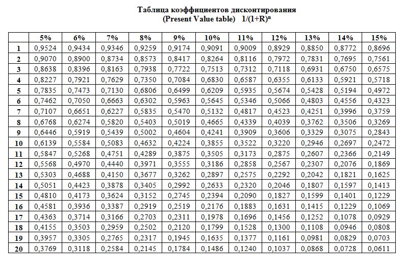
The discount factor 1/(1+R) n, as can be seen from the formula itself, depends on the interest rate and the number of time periods. In order not to calculate it each time using the discounting formula, use a table showing the values ​​of the coefficient depending on the percentage of the rate and the number of time periods. It is sometimes called a "discount table", although this is not the correct term. This discount factor table, which are calculated, as a rule, accurate to the fourth decimal place.

Using this table of discount factors is very simple: if you know the discount rate and the number of periods, for example, 10% and 5 years, then at the intersection of the corresponding columns you will find the coefficient you need.

Example 3. Let's look at a simple example. Let's say you need to choose between two options:

• A) get $100,000 today
• B) or $150,000 in one amount exactly in 5 years

What to choose?

If you know that the bank rate on 5-year deposits is 10%, then you can easily calculate what the amount of $150,000 due in 5 years is equal to today.

The corresponding discount factor in the table is 0.6209 (the cell at the intersection of the 5 years row and the 10% column). 0.6209 means that 62.09 cents received today equals $1 received in 5 years (at a 10% interest rate). Simple proportion:

So $150,000*0.6209 = 93.135.

93,135 is the discounted (present) value of the amount of $150,000 to be received in 5 years.

It's less than $100,000 today. In this case, a bird in the hand is really better than a pie in the sky. If we take $100,000 today and put it on deposit in a bank at 10% per annum, then in 5 years we will receive: 100,000*1.10*1.10*1.10*1.10*1.10 = 100,000*( 1.10) 5 = $161,050. This is a more profitable option.

To simplify this calculation (calculating future value given today's value), you can also use a coefficient table. By analogy with the discounting table, this table can be called a table of increment (accretion) factors. You can build such a table yourself in Excel if you use the formula to calculate the increment factor: (1+R)n.

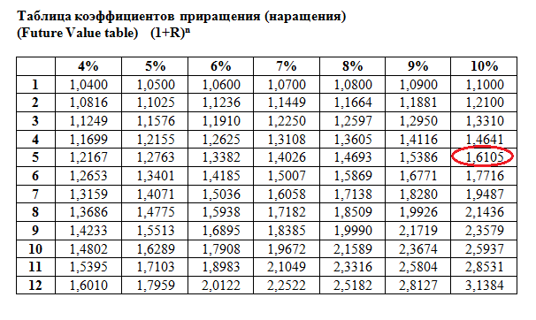From this table it can be seen that $1 today at a rate of 10% will cost $1.6105 in 5 years.

Using such a table, it will be easy to calculate how much money you need to put in the bank today if you want to receive a certain amount in the future (without replenishing the deposit). A slightly more complicated situation arises when you not only want to deposit money today, but also intend to add a certain amount to your deposit every year. How to calculate this, read the next article. It's called annuity formula.

A philosophical digression for those who have read this far

Discounting is based on the famous postulate "time is money". If you think about it, this illustration has a very deep meaning. Plant an apple tree today and in a few years your apple tree will grow and you will be picking apples for years to come. And if you don’t plant an apple tree today, then in the future you will never try apples.

All we need is to decide: to plant a tree, start our own business, take the path leading to the fulfillment of our dreams. The sooner we begin to act, the greater the harvest we will get at the end of the journey. We need to turn the time we have in our lives into results.

“The seeds of flowers that will bloom tomorrow are planted today.” That's what the Chinese say.

If you dream about something, don't listen to those who discourage you or question your future success. Don't wait for a lucky coincidence of circumstances, start as early as possible. Turn the time of your life into results.

Large table of discount rates (opens in a new window):

Investing means investing free financial resources today in order to obtain stable cash flows in the future. How not to make a mistake and not only return the invested funds, but also get a profit from the investment?

This article provides not only the formula and definition of IRR, but there are examples of calculations of this indicator (in Excel, graphical) and interpretation of the results obtained. Two examples from life that every person encounters

At its core, the discount rate when analyzing investment projects is the interest rate at which the investor attracts financing. How to calculate it?

The concept of discount rate is used to reduce the current value to the future. The discount rate is the interest rate used to convert future financial flows into a single present value.

The discount rate coefficient is calculated in different ways depending on the task being set. And the heads of companies or individual departments in modern business are faced with completely different tasks:

• implementation of investment analysis;
• business planning;
• business valuation.

For all these areas, the basis is the discount rate (its calculation), since the determination of this indicator directly affects decision-making regarding the investment of funds, the valuation of a company or individual types of business.

Discount rate from an economic point of view

Discounting determines the cash flow (its value) that relates to periods in the future (that is, future earnings at the present time). In order to correctly estimate future income, it is necessary to have information about forecasts of the following indicators:

• investments;
• expenses;
• revenue;
• capital structure;
• residual value of the property;
• discount rate.

The main purpose of the discount rate indicator is to assess the effectiveness of investments. This indicator implies a rate of return per 1 ruble. invested capital.

The discount rate, the calculation of which determines the required amount of investment to generate future income, is a key indicator when choosing investment projects.

The discount rate reflects the cost of money, taking into account temporary factors and risks. If we talk about specifics, then this rate rather reflects an individual assessment.

An example of selecting investment projects using a discount rate factor

Two projects A and C are proposed for consideration. At the initial stage, both projects require an investment of 1000 rubles; there is no need for other costs. If you invest in project A, you can receive an income of 1000 rubles annually. If you implement project C, then at the end of the first and second years the income will be 600 rubles, and at the end of the third - 2200 rubles. It is necessary to select a project, 20% per annum is the estimated discount rate.

NPV (current value of projects A and C) is calculated using the formula.

Ct - cash flows for the period from the first to the T years;

Co - initial investment - 1000 rubles;

r - discount rate - 20%.

NPV A = - 1000 = 1106 rub.;

NPV C = - 1000 = 1190 rub.

So, it turns out that it is more profitable for the investor to choose project C. However, if the current discount rate were 30%, then the cost of the projects would be almost the same - 816 and 818 rubles.

This example demonstrates that the investor's decision depends entirely on the discount rate.

Various methods for calculating the discount rate are proposed for consideration. In this article they will be considered objectively in descending order.

Weighted average cost of capital

Most often, when carrying out investment calculations, the discount rate is determined as the weighted average cost of capital, taking into account the cost indicators of shareholder (equity) capital and loans. This is the most objective way to calculate the discount rate for financial flows. Its only drawback is that not all companies can practically use it.

In order to value equity capital, the Long-Term Asset Pricing Model (CAPM) is used.

At the end of the twentieth century, American economists John Graham and Campbell Harvey surveyed 392 directors and financial managers of enterprises in various fields of activity to determine how they make decisions and what they pay attention to first. As a result of the survey, it was revealed that the academic theory is most used, or more precisely, the majority of companies calculate their equity capital using the CAPM model.

Cost of equity (calculation formula)

When calculating the cost of equity capital, the discount rate is considered differently.

Re is the rate of return, or, otherwise, the discount rate for equity capital, calculated as follows:

Re = rf + ?(rm - rf).

Where are the components of the discount rate:

• rf - risk-free rate of return;
• ? - a coefficient that determines how the price of a firm’s shares changes in comparison with changes in share prices for all firms in a given market segment;
• rm - average market rate of return on the stock market;
• (rm - rf) - premium for market risk.

Different countries take different approaches to determining the components of the model. Much in the choice depends on the general government attitude towards calculation. Each of these indicators is important to study and understand separately; this is how cash flow can be determined. Therefore, the elements of the “Valuation of Long-Term Assets” model will be discussed in more detail below. The objectivity of each component was also assessed and the discount rate was assessed.

Components of the model

The rf indicator represents the rate of return on investment in assets without risk. Risk-free assets are those in which the risk of investing is zero. These mainly include government securities. Discount rate risks are calculated differently in different countries. So, in the USA, for example, treasury bills are considered risk-free assets. In our country, for example, such assets are Russia-30 (Russian Eurobonds), the maturity of which is 30 years. Information on the profitability of these securities is presented in most economic and financial publications, such as the Vedomosti newspaper, Kommersant, and The Moscow Times.

A coefficient with a question mark in the model implies sensitivity to changes in the systematic market risk of the return on securities of a particular company. So, if the indicator is equal to one, then changes in the value of shares of this company completely coincide with changes in the market. If?-coefficient = 1.3, then with a general rise in the market, the price of shares of this company is expected to grow 30% faster than the market. And correspondingly vice versa.

In countries where the stock market is developed, the ?-coefficient is calculated by specialized information and analytical agencies, investment and consulting companies, and this information is published in specialized periodicals that analyze stock markets and financial directories.

The indicator rm - rf, which is a premium for market risk, represents the amount by which the average market rate of return on the stock market for a long time exceeded the rate of return on risk-free securities. Its calculation is based on statistical data on market premiums over a long period.

Calculating the weighted average cost of capital

If, when financing a project, they attract not only their own funds, but also borrowed funds, then the income received from this project should compensate not only the risks associated with investing their own funds, but also the funds spent on obtaining borrowed capital. To take into account the cost of both equity and debt capital, the weighted average cost of capital is used, the formula for calculation is below.

To calculate the discount rate, the CAPM model is used. Re is the rate of return on equity (shareholder) capital.

D is the market value of debt capital. Practically represents the amount of borrowings of the company according to the financial statements. If such data are not available, then the standard debt-to-equity ratio of similar firms is used.

E is the market value of share capital (equity). Obtained by multiplying the firm's total number of common shares by the price per share.

Rd represents the firm's rate of return on debt capital. Such costs include information on bank interest on loans and bonds of a corporate company. In addition, the valuation of borrowed capital is adjusted taking into account the income tax rate. According to tax legislation, interest on loans and borrowings is charged to the cost of goods, thus reducing the tax base.

Tc - income tax.

WACC model: calculation example

Using the WACC model, the discount rate for company X is specified.

The calculation formula (an example was given when calculating the weighted average cost of capital) requires the following input indicators.

• Rf = 10%;
• ? = 0,90;
• (Rm - Rf) = 8.76%.

So, equity capital (its profitability) is equal to:

Re = 10% + 0.90 x 8.76% = 17.88%.

E/V = 80% - the share occupied by the market value of share capital in the total cost of capital of company X.

Rd = 12% - weighted average level of costs for raising borrowed funds for company X.

D/V = 20% - the share of the company's borrowed funds in the total cost of capital.

tc = 25% - profit tax indicator.

Thus, WACC = 80% x 17.88% + 20% x 12% x (1 - 0.25) = 14.32%.

As noted above, certain methods for calculating discount rates are not suitable for all companies. And this technique is exactly this case.

Firms may be better off choosing other methods for calculating the discount rate unless the company is a public limited company and its shares are not traded on a stock exchange. Or if the company does not have enough statistics to determine the?-coefficient and it is impossible to find similar companies.

Cumulative assessment methodology

The most common and most often used method in practice is the cumulative method, which also uses it to estimate the discount rate. Calculation using this method suggests the following conclusions:

• if investments did not involve risk, then investors would require a risk-free return on their capital (the rate of return would correspond to the rate of return on investments in risk-free assets);
• The higher an investor assesses the risk of a project, the higher the requirements they place on its profitability.

Therefore, when the discount rate is calculated, the so-called risk premium must be taken into account. Accordingly, the discount rate will be calculated as follows:

R = Rf + R1 + ... + Rt,

where R is the discount rate;

Rf - risk-free rate of return;

R1 + ... + Rt - risk premiums for different risk factors.

It is practically possible to determine one or another risk factor, as well as the value of each risk premium, only by expert means.

When determining the effectiveness of investment projects, the cumulative method of calculating the discount rate recommends taking into account 3 types of risk:

• risk arising from the dishonesty of project players;
• risk arising from non-receipt of planned income;
• country risk.

The value of country risk is indicated in various ratings, which are compiled by special rating firms and consulting companies (for example, BERI). The fact of unreliability of project participants is compensated by a risk premium; the recommended indicator is no more than 5%. The risk arising from non-receipt of planned income is established in accordance with the goals of the project. There is a special calculation table.

Discount rates estimated by this method are quite subjective (too dependent on expert risk assessment). They are also much less accurate than the calculation method based on the “Valuation of Long-Term Assets” model.

Expert assessment and other calculation methods

The simplest way to calculate the discount rate and quite popular in real life is to set it using the expert method, with reference to the requirements of investors.

It is clear that for private investors, a calculation based on formulas cannot be the only way to make a decision regarding the correctness of setting the discount rate for a project/business. Any mathematical models can only approximately assess the reality of the situation. Investors, relying on their own knowledge and experience, are able to determine a sufficient profitability for the project and rely on it as a discount rate when making calculations. But for adequate sensations, an investor must understand the market very well and have extensive experience.

However, we must assume that the expert methodology is the least accurate and may well distort the results of business (project) assessment. Therefore, it is recommended that when determining the discount rate using expert or cumulative methods, it is mandatory to analyze the sensitivity of the project to changes in the discount rate. In this case, investors will have the most accurate assessment possible.

Of course, alternative methods for calculating the discount rate exist and are used. For example, the theory of arbitrage pricing, the dividend growth model. But these theories are very difficult to understand and are rarely applied in practice.

Application of discount rate in real life

In conclusion, I would like to note that most companies in the course of their activities need to determine the discount rate. It is necessary to understand that the most accurate indicator can be obtained using the WACC technique, while other methods have a significant error.

In work, you rarely have to calculate the discount rate. This is mainly associated with the evaluation of large and significant projects. Their implementation entails a change in the capital structure and stock price of the company. In such cases, the discount rate and the method of its calculation are agreed upon with the investing bank. They focus mainly on the risks obtained in similar companies and markets.

The use of certain techniques also depends on the project. In cases where industry standards, production technology, financing are clear and known, and statistical data have been accumulated, the standard discount rate established at the enterprise is used. When evaluating small and medium-sized projects, they refer to the calculation of payback periods, with an emphasis on analyzing the structure and external competitive environment. In fact, methods for calculating the discount rate of real options and cash flows are combined.

You need to be aware that the discount rate is only an intermediate link in the evaluation of projects or assets. In reality, the assessment is always subjective, the main thing is that it is logical.

There is such a mistake - economic risks are taken into account twice. So, for example, two concepts are often confused - country risk and inflation. As a result, the discount rate doubles and a contradiction appears.

There is not always a need to count. There is a special table for calculating the discount rate, which is very easy to use.

Also a good indicator is the cost of credit for a particular borrower. The setting of the discount rate may be based on the actual lending rate and the level of yield of bonds that are available on the market. After all, the profitability of a project does not exist only within its own environment; it is also influenced by the general economic situation in the market.

However, the obtained indicators also require significant adjustments related to the risk of the business (project) itself. Currently, the real options technique is used quite often, but it is very complex from a methodological point of view.

In order to take into account such risk factors as the possibility of project suspension, technology changes, market losses, project evaluation practitioners artificially inflate discount rates (up to 50%). However, there is no theory behind these numbers. Similar results can be obtained using complex calculations, in which, in any case, most of the forecast indicators would be determined subjectively.

Correctly determining the discount rate is a problem associated with the basic requirement for the information content generated in financial reporting and accounting. In other words, if there is reason to doubt whether assets or liabilities are valued correctly, and whether monetary compensation is delayed, then discounting must be applied.

When choosing a discount rate, it is important to understand that it should be as close as possible to the rate received by the borrower of the lending bank under real conditions in the existing environment.

So, the discount rate for certain assets (for example, for fixed assets) is equal to the rate at which the company would have to pay if it raised funds to purchase similar property.