NPV in Excel. NPV calculation in Excel (example)
There are many financial formulas in Excel. Let's look at the most important formulas that will allow you to calculate:
- (Net Present Value) or net present value;
- IRR of an investment project(Internal Rate of Return) or internal rate of return;
We will also consider some of the nuances and tricks of using these formulas. All calculations can be found in the attached file. The main focus is on Excel functions.
How to calculate NPV in Excel
Let's consider a conditional example: there is a project that will bring in 250,000 rubles annually for 5 years. Its implementation requires 1,000,000 rubles. - 10%.
If the cash flows reduced to the current period are greater than the invested money (NPV>0), then the project is profitable. Otherwise, no.
The NPV formula looks like this:
If the cash flows reduced to the current period are greater than the invested money (NPV>0), then the project is profitable. Otherwise no.
To calculate NPV, we will need to do the following in Excel: 
Let's add serial numbers of years: 0 – starting year, flows are reduced to it.
1, 2, 3, etc. – these are the years of project implementation. The formula in the figure performs the actions that are written above after the sum sign (Σ).
We divide the cash flow for the period by the amount of 1 and the discount rate raised to the power of the corresponding year. The calculated line represents the discounted cash flow. To get the NPV value, it is enough to find the total amount of the entire line.
It turns out “-52 303”. The project is unprofitable.
Read also:
Who will find it useful?: Let’s say your company plans to invest in a project that seems promising at first glance. It has a good net present value (NPV), a good internal rate of return (IRR). These indicators seem completely standard and generally accepted. But there are many subtleties in their calculations that affect the final figure, and sometimes the decision made. Read the article to understand the features of project evaluation by analyzing it using different techniques.
Calculating NPV using the NPV formula
To calculate NPV in Excel, it is not necessary to prepare such a table. Just use the NPV formula in Excel. Where NPV is the discount rate; range of discounted values. That is, it is enough to indicate a cell with interest and cash flows. But when using this formula out of habit, financiers often make a mistake: 
In fact, the results should be the same. Why are there different meanings here? The fact is that NPV in Excel starts discounting from the very first value. That is, it looks for present value. And the initial investment must be taken away afterwards. The correct form of the formula in our case will be as follows:

The starting investments are “removed” beyond the discounted range (red) and added (actually, subtracted: since the starting investments are already minus, D8 needs to be added) separately. Now the result is the same.
More on the topic:
How it will help: The modified internal rate of return, compared to the conventional internal rate of return, allows for a more accurate assessment of the effectiveness of investment projects in which the net cash flow changes sign several times during the life cycle. How to calculate this indicator is described in this solution.
How it will help: in order to choose the most profitable of two investment projects, you have to evaluate the effectiveness of each of them according to one or more indicators - payback period, rate of return, net present value and internal rate of return. More details on how to compare them if the projects themselves are not comparable can be found in this solution.
How to evaluate the effectiveness of an investment project in Excel using IRR
IRR is another indicator for evaluating investment projects. IRR answers the question: what should the rate be for NPV to become = 0?
IRR Formula in Excel
If the discount rate< IRR, то проект стоит принять, если нет – отказаться. Как рассчитать IRR в Excel? Очень просто: Подставляем в функцию ВСД итоговый денежный поток.

The IRR turned out to be less than the rate of return. The project is unprofitable (same conclusion as with NPV).
NPV and IRR are rightfully considered the main economic criteria. They are used both for investment evaluation of projects and for assessing the value of existing businesses. In particular, the EVA (Economic Value Added) indicator is considered a good criterion, since if calculated correctly it is equal to NPV.
Where else can you use NPV and IRR calculations in Excel?
NPV and IRR financial specialists can use it in more applied matters. For example, in resolving the issue with banks about the real lending rate. The fact is that when issuing a loan, banks calculate the amount of annuity or, in other words, a flat payment. To plan loan payments, it is important to understand how annuity is calculated.
Let's say you are going to take out a loan of 1,000,000 rubles for 5 years at 10% per annum. You will pay once a year in equal installments. We will not present the formula for calculating annuity from a textbook on financial management here. Here's the Excel formula:
PMT – discount rate; number of periods; the loan amount you take out.
There are two more optional points in the formula. The amount that should remain (zero by default) and how to calculate the amount: at the beginning of the month - set 1, at the end of the month - zero. In most cases, these items are not needed, so they can be omitted at all. The total annuity amount is determined as follows:

The amount of the annual payment is immediately minus. This amount must be paid to the bank every year. It contains two parts:
- Loan payment – we take 10% (interest on the loan) of the debt amount at the beginning of the period.
- The loan body is the difference between the annual payment and the interest payment (in Excel you can find formulas that will calculate these payments for you).
The debt at the end of the month is calculated as the difference between the debt at the beginning and the payment on the loan body. If payments are not annual, but monthly or quarterly, then the rate and period must be adjusted to these values. So if we had a payment every month, the formula for calculating the annuity would look like this:
We would divide the annual rate by 12 (resulting in a monthly rate) and take not 5 periods, but 5 12 = 60 months. We receive a monthly payment equal to 21,247 rubles.
How to check banks for honesty by calculating NPV and IRR in Excel
Any flow of loan payments implies that all outflows of money are reduced to inflows at the lending rate. In other words, if we build the cash flow from the loan we received and subsequent annuity payments, we can calculate NPV and IRR from them. NPV should take zero value, and IRR should show us the real interest rate.
When the loan and its payments are calculated correctly, the NPV taken at the same interest rate is zero. And IRR shows the same rate. When the bank makes us an offer that is impossible to refuse, and which will increase the loan rate “only” by a certain percentage, do not believe it and recalculate. I will give an example of how to calculate IRR and understand the real interest on a loan.
The bank offered insurance at “only” 2% of the loan amount per year. Do you think this is an increase of only 2%? No. The fact is that real credit decreases at the beginning of each year: 
The result shows that NPV is not zero. But the real percentage is not 10, but 12.9%. Please note that the overpayment amount has increased here. If you are confused by this, you may be offered “even more favorable conditions” - pay the overpayment now, and the rest later, in smaller payments, or, as in our example, simply pay more and then less. The amount of overpayment will not change, but the percentage will change significantly.

What has been done here? The amount of 43,797 rubles was taken from each subsequent payment and added to the first payment. If for the real sector financial mathematics about “money yesterday - money tomorrow” seems somewhat distant from life, for banks it is real profit. Therefore, they are already loading the first payment. And with the help of simple formulas you can track this and prepare the basis for further negotiations.
P.S. Don’t forget, when it comes to monthly payments, multiply by 12.
And what formulas are used to calculate this indicator, but it requires simple tools at hand that allow you to calculate NPV faster than manually or using conventional calculators.
A multifunctional environment helps them, allowing them to calculate NPV using tabular data or using special functions.
Let's look at a hypothetical example, which we will solve by applying the formula for calculating NPV that we already know, and then we will repeat our calculations using the capabilities of Excel.
Problem of finding NPV
Example. The initial ones in A are 10,000 rubles. Annual – 10%. The dynamics of revenues from years 1 to 10 are presented in the table below:
| Period | Tributaries | Outflows |
| 0 | 10000 | |
| 1 | 1100 | |
| 2 | 1200 | |
| 3 | 1300 | |
| 4 | 1450 | |
| 5 | 1600 | |
| 6 | 1720 | |
| 7 | 1860 | |
| 8 | 2200 | |
| 9 | 2500 | |
| 10 | 3600 |
For clarity, the corresponding data can be presented graphically:
Figure 1. Graphical representation of the initial data for calculating NPV
Standard solution. To solve the problem, we will use the NPV formula we already know:

We simply substitute known values into it, which we then sum. For these calculations we will need a calculator:
NPV = -10000/1,1 0 + 1100/1,1 1 + 1200/1,1 2 + 1300/1,1 3 + 1450/1,1 4 + 1600/1,1 5 + 1720/1,1 6 + 1860/1,1 7 + 2200/1,1 8 + 2500/1,1 9 + 3600/1,1 10 = 352.1738 rubles.
NPV calculation in Excel (tabular example)
We can solve this same example by organizing the relevant data in the form of an Excel table.
It should look something like this:

Figure 2. Layout of example data on an Excel sheet
In order to get the desired result, we must fill in the corresponding cells with the necessary formulas.
| Cell | Formula |
| E4 | =1/DEGREE(1+$F$2/100;B4) |
| E5 | =1/DEGREE(1+$F$2/100;B5) |
| E6 | =1/DEGREE(1+$F$2/100;B6) |
| E7 | =1/DEGREE(1+$F$2/100;B7) |
| E8 | =1/DEGREE(1+$F$2/100;B8) |
| E9 | =1/DEGREE(1+$F$2/100;B9) |
| E10 | =1/DEGREE(1+$F$2/100;B10) |
| E11 | =1/DEGREE(1+$F$2/100;B11) |
| E12 | =1/DEGREE(1+$F$2/100;B12) |
| E13 | =1/DEGREE(1+$F$2/100;B13) |
| E14 | =1/DEGREE(1+$F$2/100;B14) |
| F4 | =(C4-D4)*E4 |
| F5 | =(C5-D5)*E5 |
| F6 | =(C6-D6)*E6 |
| F7 | =(C7-D7)*E7 |
| F8 | =(C8-D8)*E8 |
| F9 | =(C9-D9)*E9 |
| F10 | =(C10-D10)*E10 |
| F11 | =(C11-D11)*E11 |
| F12 | =(C12-D12)*E12 |
| F13 | =(C13-D13)*E13 |
| F14 | =(C14-D14)*E14 |
| F15 | =SUM(F4:F14) |
As a result, in cell F15 we get the desired NPV value equal to 352.1738.
It takes 3-4 minutes to create such a table. Excel allows you to find the desired NPV value faster.
NPV calculation in Excel (NPV function)
Place the formula in cell B17 (or any other cell):
NPV(F2/100;C5:C14)-D14
We will instantly receive the exact NPV value in rubles (352.1738 rubles).

Figure 3. NPV calculation using Excel NPV formula
Our formula refers to cells F2 (we have an interest rate of 10% there; to use it in the NPV function, we need to divide it by 100), the value range C5:C14, where the data on inflows is located, and cell D14, which contains the size of the initial
IRR (Internal Rate of Return), or IRR, is an indicator of the internal rate of return of an investment project. Often used to compare different proposals for growth prospects and profitability. The higher the IRR, the greater the growth prospects for a given project. Let's calculate the GNI interest rate in Excel.
Economic meaning of the indicator
Other names: internal rate of return (profit, discount), internal rate of return (efficiency), internal rate.
The IRR coefficient shows the minimum level of profitability of an investment project. In other words: this is the interest rate at which the net present value is zero.
Formula for calculating the indicator manually:
- CFt – cash flow for a certain period of time t;
- IC – investments in the project at the entry (launch) stage;
- t – time period.
In practice, the IRR coefficient is often compared with the weighted average cost of capital:
- IRR is higher - this project should be carefully considered.
- The IRR is lower – it is not advisable to invest in the development of the project.
- The indicators are equal - the minimum acceptable level (the company needs to adjust its cash flow).
IRR is often compared as a percentage of a bank deposit. If the interest on the deposit is higher, then it is better to look for another investment project.
Example of IRR calculation in Excel
- range of values – a link to cells with numeric arguments for which you need to calculate the internal rate of return (at least one cash flow must have a negative value);
- guess – a value that is supposedly close to the value of the IRR (the argument is optional; but if the function throws an error, the argument must be specified).
Let's take some conventional numbers:

The initial costs were 150,000, so this numerical value was included in the table with a minus sign. Now let's find the IRR. Calculation formula in Excel:

Calculations showed that the internal rate of return of the investment project is 11%. For further analysis, the value is compared with the interest rate of a bank deposit, or the cost of capital of a given project, or the IRR of another investment project.
We calculated IRR for regular cash inflows. For unsystematic receipts, it is impossible to use the VSD function, because The discount rate for each cash flow will change. Let's solve the problem using the function NET.
Let's modify the table with the source data for example:

Required arguments for the NETIR function:
- values – cash flows;
- dates – an array of dates in the appropriate format.
Formula for calculating IRR for non-systematic payments:

A significant drawback of the previous two functions is the unrealistic assumption of the reinvestment rate. To correctly account for the reinvestment assumption, it is recommended to use the MVSD function.
Arguments:
- values – payments;
- financing rate – interest paid on funds in circulation;
- reinvestment rate.
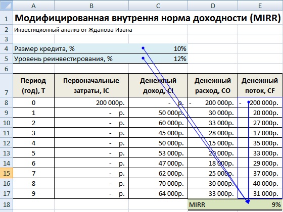
Let's assume that the discount rate is 10%. It is possible to reinvest the income received at a rate of 7% per annum. Let's calculate the modified internal rate of return:

The resulting rate of profit is three times less than the previous result. And lower financing rates. Therefore, the profitability of this project is questionable.
Graphical method for calculating IRR in Excel
The IRR value can be found graphically by plotting the net present value (NPV) versus the discount rate. NPV is one of the methods for evaluating an investment project, which is based on the discounted cash flow methodology.
For example, let’s take a project with the following cash flow structure:

To calculate NPV in Excel, you can use the NPV function:

Since the first cash flow occurred in period zero, it should not be included in the array of values. The initial investment must be added to the value calculated by the NPV function.
The function discounted cash flows of periods 1-4 at a rate of 10% (0.10). When analyzing a new investment project, it is impossible to accurately determine the discount rate and all cash flows. It makes sense to look at the dependence of NPV on these indicators. In particular, on the cost of capital (discount rate).
Let's calculate NPV for different discount rates:

Let's look at the results on the graph:

Let us recall that IRR is the discount rate at which the NPV of the analyzed project is equal to zero. Consequently, the point of intersection of the NPV graph with the x-axis is the internal profitability of the enterprise.
Let's analyze such an indicator as the internal rate of return of an investment project, determine the economic meaning and consider in detail an example of its calculation using Excel.
Internal rate of return of an investment project (IRR). Definition
Internal rate of return(English) InternalRateofReturn,IRR, internal rate of return, internal rate, internal rate of return, internal discount rate, internal efficiency ratio, internal payback ratio) – a coefficient showing the maximum acceptable risk for an investment project or the minimum acceptable level of profitability. The internal rate of return is equal to the discount rate at which there is no net present value, that is, zero.
Internal rate of return calculation formula
CFt( Cash Flow) – cash flow in time period t;
IC( Invest Capital) – investment costs for the project in the initial period (also cash flow CF 0 = IC).
t – time period.
 |
★ |
Application of internal rate of return
The indicator is used to assess the attractiveness of an investment project or for comparative analysis with other projects. To do this, IRR is compared with the effective discount rate, that is, with the required level of profitability of the project (r). For this level in practice, the weighted average cost of capital is often used ( WeightAverageCost ofCapital, WACC).
| MeaningIRR | Comments |
| IRR>WACC | An investment project has an internal rate of return higher than the cost of equity and borrowed capital. This project should be accepted for further analysis |
IRR | The investment project has a rate of return lower than the cost of capital, this indicates the inappropriateness of investing in it |
|
| IRR=WACC | The internal return of the project is equal to the cost of capital, the project is at the minimum acceptable level and cash flow adjustments should be made and cash flows increased |
| IRR 1 >IRR 2 | Investment project (1) has greater investment potential than (2) |
It should be noted that instead of the WACC comparison criterion, there can be any other barrier level of investment costs, which can be calculated using methods for estimating the discount rate. These methods are discussed in detail in the article "". A simple practical example would be to compare the IRR with the risk-free interest rate on a bank deposit. So if an investment project has IRR = 10%, and the interest on the deposit = 16%, then this project should be rejected.
The internal rate of return (IRR) is closely related to the net present value (NPV). The figure below shows the relationship between the size of IRR and NPV; an increase in the rate of return leads to a decrease in income from the investment project.

Master class: “How to calculate the internal rate of return of a business plan”
Calculation of internal rate of return (IRR) using an example in Excel
Let's look at an example of calculating the internal rate of return using Excel, and look at two methods of construction using a function and using the “Solution Search” add-in.
Example of calculating IRR in Excel using the built-in function
The program has a built-in financial function that allows you to quickly calculate this indicator - IRR (internal discount rate). It should be noted that this formula will only work when there is at least one positive and one negative cash flow. The calculation formula in Excel will look like this:
Internal rate of return (E16)=VSD(E6:E15)

Internal rate of return. Calculation in Excel using built-in formula
As a result, we found that the internal rate of return is 6%; then, to conduct an investment analysis, the obtained value must be compared with the cost of capital (WACC) of this project.
|
★ (calculation of Sharpe, Sortino, Treynor, Kalmar, Modiglanca beta, VaR) + forecasting course movements |
Example of calculating IRR using the “Solution Search” add-on
The second calculation option involves using the “Solution Search” add-on to find the optimal value of the discount rate for NPV=0. To do this, you need to calculate net present value (NPV).
The figure below shows the formulas for calculating discounted cash flow by year, the sum of which gives net present value. The formula for calculating discounted cash flow (DCF) is as follows:
Discounted cash flow (F)=E7/(1+$F$17)^A7
Net present value (NPV)=SUM(F7:F15)-B6
The figure below shows the initial view for calculating IRR. You will notice that the discount rate used to calculate NPV refers to a cell that has no data (it is set to 0).

Internal rate of return (IRR) and NPV. Calculation in Excel using an add-in
Now our task is to find, based on optimization using the “Search for Solutions” add-on, the value of the discount rate (IRR) at which the NPV of the project will be equal to zero. To do this, open the “Data” section in the main menu and “Search for solutions” in it.

When you click in the window that appears, fill in the lines “Set target cell” - this is the formula for calculating NPV, then select the value of this cell equal to 0. The variable parameter will be the cell with the value of the internal rate of return (IRR). The figure below shows an example of a calculation using the Solution Search add-on.

Finding the IRR value for NPV=0
After optimization, the program will fill our empty cell (F17) with the value of the discount rate at which the net present value is zero. In our case, it turned out to be 6%, the result completely coincides with the calculation using the built-in formula in Excel.

The result of calculating the internal rate of return (IRR)
Calculation of internal rate of return in Excel for unsystematic receipts
In practice, it often happens that funds do not arrive periodically. As a result, the discount rate for each cash flow will change, making it impossible to use the IRR formula in Excel. To solve this problem, another financial formula is used: NET INDOH (). This formula includes an array of dates and cash flows. The calculation formula will be as follows:
NETINDOH(E6:E15;A6:A15;0)

Calculation of internal rate of return in Excel for non-systematic payments
Modified internal rate of return (MIRR)
Also used in investment analysis modified internal rate of return (Modified InternalRateofReturn,MIRR) – this indicator reflects the minimum internal level of profitability of the project when reinvesting in the project. This project uses interest rates received from reinvesting capital. The formula for calculating the modified internal rate of return is as follows:

MIRR – internal rate of return of an investment project;
COF t – cash outflow during time periods t;
CIFt – cash inflow;
r is the discount rate, which can be calculated as the weighted average cost of capital WACC;
d – interest rate of capital reinvestment;
n – number of time periods.
Calculation of modified internal rate of return in Excel
To calculate this modification of the internal rate of return, you can use the built-in Excel function, which uses, in addition to cash flows, the size of the discount rate and the level of return on reinvestment. The formula for calculating the indicator is presented below:
MIRR =MIRR(E8:E17,C4,C5)
Advantages and Disadvantages of Internal Rate of Return (IRR)
Let's consider advantages of the indicator internal rate of return for project evaluation.
Firstly, the ability to compare various investment projects with each other in terms of the degree of attractiveness and efficiency of capital use. For example, comparison with the return on risk-free assets.
Secondly, the ability to compare different investment projects with different investment horizons.
TO shortcomings of the indicator include:
First, the disadvantages of estimating internal rate of return are the difficulty of predicting future cash payments. The amount of planned payments is influenced by many risk factors, the impact of which is difficult to objectively assess.
Secondly, the IRR indicator does not reflect the amount of reinvestment in the project (this shortcoming is resolved in the modified internal rate of return MIRR).
Third, the inability to reflect the absolute amount of cash received from the investment.
Summary
In this article, we examined the formula for calculating the internal rate of return (IRR), and examined in detail two ways to construct this investment indicator using Excel: based on built-in functions and the “Solution Search” add-in for systematic and unsystematic cash flows. It was highlighted that the internal rate of return is the second most important indicator for evaluating investment projects after net present value (NPV). A variation of IRR is its modification MIRR, which also takes into account the return on capital reinvestment.
NPV (abbreviation in English - Net Present Value), in Russian this indicator has several variations of the name, among them:
- net present value (abbreviated NPV) is the most common name and abbreviation, even the formula in Excel is called exactly that;
- net present value (abbreviated NPV) - the name is due to the fact that cash flows are discounted and only then summed up;
- net present value (abbreviated NPV) - the name is due to the fact that all income and losses from activities due to discounting are, as it were, reduced to the current value of money (after all, from the point of view of economics, if we earn 1,000 rubles and then actually receive less than if we received the same amount, but now).
NPV is an indicator of the profit that participants in an investment project will receive. Mathematically, this indicator is found by discounting the values of net cash flow (regardless of whether it is negative or positive).
Net present value can be found for any period of time of the project since its beginning (for 5 years, for 7 years, for 10 years, and so on) depending on the need for calculation.
What is it needed for
NPV is one of the indicators of project efficiency, along with IRR, simple and discounted payback period. It is needed to:
- understand what kind of income the project will bring, whether it will pay off in principle or is it unprofitable, when it will be able to pay off and how much money it will bring at a particular point in time;
- to compare investment projects (if there are a number of projects, but there is not enough money for everyone, then projects with the greatest opportunity to earn money, i.e. the highest NPV, are taken).
Calculation formula
To calculate the indicator, the following formula is used:
- CF - the amount of net cash flow over a period of time (month, quarter, year, etc.);
- t is the time period for which the net cash flow is taken;
- N is the number of periods for which the investment project is calculated;
- i is the discount rate taken into account in this project.
Calculation example
To consider an example of calculating the NPV indicator, let's take a simplified project for the construction of a small office building. According to the investment project, the following cash flows are planned (thousand rubles):
| Article | 1 year | 2 year | 3 year | 4 year | 5 year |
| Investments in the project | 100 000 | ||||
| Operating income | 35 000 | 37 000 | 38 000 | 40 000 | |
| Operating expenses | 4 000 | 4 500 | 5 000 | 5 500 | |
| Net cash flow | - 100 000 | 31 000 | 32 500 | 33 000 | 34 500 |
The project discount rate is 10%.
Substituting into the formula the values of net cash flow for each period (where negative cash flow is obtained, we put it with a minus sign) and adjusting them taking into account the discount rate, we get the following result:
NPV = - 100,000 / 1.1 + 31,000 / 1.1 2 + 32,500 / 1.1 3 + 33,000 / 1.1 4 + 34,500 / 1.1 5 = 3,089.70
To illustrate how NPV is calculated in Excel, let's look at the previous example by entering it into tables. The calculation can be done in two ways
- Excel has an NPV formula that calculates the net present value, to do this you need to specify the discount rate (without the percent sign) and highlight the range of the net cash flow. The formula looks like this: = NPV (percent; range of net cash flow).
- You can create an additional table yourself where you can discount the cash flow and sum it up.
Below in the figure we have shown both calculations (the first shows the formulas, the second the calculation results):


As you can see, both calculation methods lead to the same result, which means that depending on what you are more comfortable using, you can use any of the presented calculation options.